Theory

The dynamic capillaroscopy option enables capillary blood cell velocity to measured from live or recorded video using a spatial correlation technique.

Measurements can be made in real time, directly from the subject. However, it is usually more convenient to record onto good quality video tape or, for best quality, directly into the computer memory, or for longer sequences, directly to the hard disk. This also allows more than one vessel to be measured from the same image sequence. Note that the digitised video is not compressed, and will use about 10 Mbyte per second for a full frame.

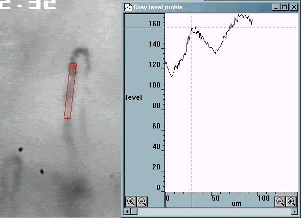
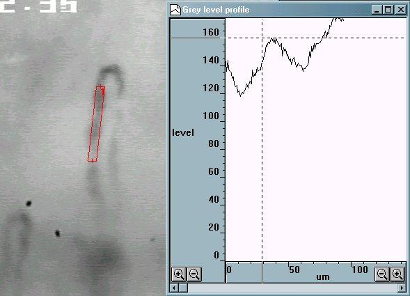
Velocity is measured by using the mouse to draw a line along the vessel. The vessel can have any orientation, and does not even need to be straight, although straight vessels are more likely to give good results. The line thickness can be adjusted so that it covers the width of the capillary. This gives an average of the pattern over the whole width. i.e. the image of the vessel is projected onto a 1 pixel thick line. Note that the image itself has already effectively projected 3D into a 2D image (thicker vessels appear darker), and the averaging across the width of the vessel reduces the 2D information down to 1 dimension.

The grey level profile along the line is taken for each field every 1/50th of a second (1/60th second for NTSC based systems). Note that standard video formats have 25 (or 30) frames per second, but each frame is made from 2 interlaced fields. Even numbered lines make the even field, and odd numbered lines make the odd field. Usually, each field is captured seperately and then sent whilst the next field is being captured.

The grey level pattern along each line is compared to the pattern from the next field (or several fields later for very low velocities).

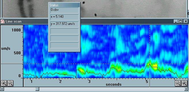
The comparison is performed by calculating the correlation coefficient for every possible shift of the previous grey level profile relative to the new profile. The shift which produces the highest correlation, and which can be seen as the peak in the correlation (the y scale is multiplied by 1000) in the following figure, indicates the distance that the pattern travelled between the two grey level profile measurements.

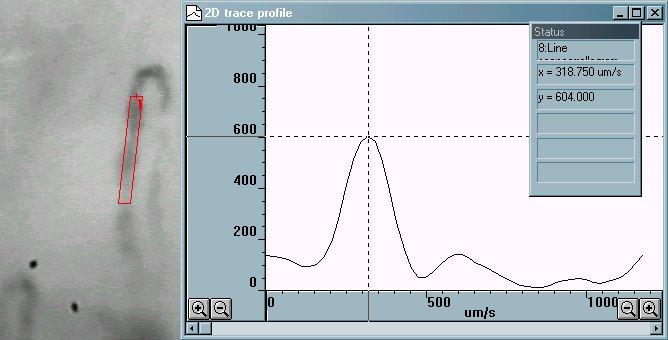
Since the time laspe between the two grey level profiles is known (ie 1/50th second) the velocity is easily calculated. CapiScope displays the correlation, along with the velocity trace (cbv) as a colour map, showing red for a high correlation through to blue for low correlation. If the correlation is below a preset limit then it is rejected, and a zero cbv value is set at that point.