Charts
Introduction to charts
Charts are documents that contain data in the form of traces. A chart can contain many traces. Traces can be moved between charts or duplicated, via the clipboard. To copy a section of a trace to another chart, first select a section of the trace, copy to the clipboard, then paste into the other chart.
Traces can be smoothed (low pass filtered) and averaged. The results of average calculations are placed in Results documents. These can be saved to disc. Selected results from a Results document can be copied to a spreadsheet such as Excel via the clipboard.
Axes
Using the mouse
The x and y scales can be altered by clicking on the  or
or buttons on the
respective axes.
buttons on the
respective axes.
The view of the data can be scrolled along the x axis by using the ScrollBar on the bottom of the Trace window.
The left and right arrow buttons on the scroll bar scroll all the traces by one pixel.
Clicking with the left button on either side of the scroll box, the traces are scrolled 3/4 of the visible view. Dragging the scroll box scrolls the traces accordingly.
The y scale can be offset by clicking on the y axis with the left mouse button and dragging up or down. The y axis controls only effects the traces in the same Y group as the currently active trace.
Using the Keyboard
The x axis scale can be increased or decreased by using the '+' and '-' keys.
Use the up and down cursor keys for the y axis scale.
Use the Page Up, Page Down, Home, End, cursor left and right keys to scroll along the x axis.
See Keyboard below.
Traces
A trace window or file can contain more than one trace. Each trace has its own y axis, but only one y axis is visible at any one time. To activate a trace click on it using the left mouse button, or use the TAB key to activate the next trace. The currently active trace is indicated by its name displayed in the Status
Trace Properties
The trace properties can be altered by clicking the trace with the right mouse button or using the Trace Properties command in the edit menu. A Trace Properties Dialog box allows properties such as the trace name and trace colour to be altered. Note that some colours may not be printed on non-colour printers.
Selecting Trace Data
Click on the trace to select data by using the left mouse button. Drag the mouse whilst holding the left button down. Selected data will be highlighted.
Use the Copy Tool Bar button, <CTRL><Insert> keys or <CTRL>C keys to copy the data into the clipboard. In the current version this is stored in a private format which can only be used by CapiScope.
Use the '=' Tool Bar button to calculate averages etc. the results will be appended to the last activated Results window, or if no results windows are open then a new results file will be created.
Adding a Trace to a File
Use the Paste Tool Bar button or <SHIFT><Insert>, or <CTRL>V keys to insert data from the clipboard into the currently active trace window. If the window contains a marked selection then the data will be copied to that location, otherwise it is copied to the start.
Display Rate
Data can be displayed at any rate independent of the data rate. Additionally two or more windows can be used to show the data at different rates. For example use Window|Duplicate Window to produce two views of the CAM1 monitor window. One could be set to a slow display rate to show long term trends whilst using the other window at a fast display rate to show the pulsatile component.
Display rate is controlled by using the x axis magnify/minify buttons.
Edit
Edit Copy command
Use this command to copy selected data from the active trace onto the clipboard. This command is unavailable if there is no data currently selected.
Copying data to the clipboard replaces the contents previously stored there.
Note that when copying large 2D colour traces, there will be two copies in memory. Also if this is then pasted into another document, there could be three copies in memory. This could cause the system to become very sluggish. It is a good idea to copy a small section of a line trace into the clipboard to release at least one copy from memory.
Shortcuts: Tool Bar  ; Keys: CTRLC, CTRLInsert
Edit Cut command
Use this command to remove the currently selected data from the active trace or the whole active trace if there is no data currently selected and put it on the clipboard.
The 'cut' data is set to zero in the trace if a selection was used (ie memory is still used).
The active trace is removed from the chart if no selection was made.
Cutting data to the clipboard replaces the contents previously stored there.
Shortcuts: Tool Bar .Keys: CTRLX; ShiftDelete
Edit Delete Command
Use this command to remove the currently active trace from the chart.
If part of a trace is selected, then the selection is set to zero, no memory is freed.
All unsaved data will be lost forever.
Not available in the monitor window.
Edit Paste command
Use this command to insert a copy of the clipboard contents at the insertion point or the beginning of the Chart (t=0) if there is no selection. This command is unavailable if the clipboard is empty.
Traces cannot be pasted into the Monitor window.
Shortcuts: Tool Bar: Keys: CTRLV,SHIFTInsert
Markers
Event Markers
Event Markers are small flags which can be used to mark events, artifacts, or Captured Images using CapiScope during a recording. Markers can also be added later to highlight a feature.
An Event Marker contains a label, which is shown on the flag, and a notelet, which can contain more detailed information. Event Markers are stored with the Chart, and are also Copied / Pasted to/from the clipboard together with the active trace.
Image Markers contain the filename of the captured image in the notelet.
Markers are added to a recording by pressing the space bar. This will generate a marker with a sequential number for the label, and will add the time and date to the notelet.
Alternatively, a marker can be created by pressing any key, the character from that key will be used for the label, and the time and date will be added to the notelet.
Image markers are added by pressing the F4 function key.
Markers can be added to a Chart by switching to Marker Mode and then clicking with the left mouse button to place a marker at the current cursor position.
Any marker can be edited by clicking on it with the right mouse button. This will open the Edit Marker box.
Markers can be edited as soon as they are created by enabling the Edit New Marks option in the Settings menu.
Edit Marker Dialog
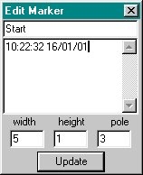
This dialog allows the properties of the selected Event Marker to be edited.
The first line is the text displayed on the Event Marker flag, and the large edit box allows more descriptive notes to be added and saved with the marker. (Use <Ctrl> <Return> to add a newline to the note).
The marker is not updated until the Update button is clicked.
The dialog will show the properties of any newly selected marker if a different marker is selected whilst the Edit Marker Dialog is open. This makes it quicker to view the contents of many markers.
Edit New Marks
Enable this option to always open up the Edit Markers dialog box whenever a new marker is created. This is particularly useful if descriptive markers are required during recording. The suggested procedure is:
(i) Press the spacebar to create the new marker. The markers position is set to the time at which the spacebar is pressed.
(ii) Type in the label for the new marker and press return.
The only disadvantages using this method are that one or two data points may be lost whilst Windows creates the Edit Markers dialog box, and that the Doppler Spectrum trace is not redrawn when the dialog box is closed (WCAM1 disables the Doppler trace redrawing whilst recording to minimise lost data).
Note the new marker is not redrawn with the new label until recording is stopped.
Marker Mode
Use this to enable/disable the marker mode. When enabled, clicking the left mouse button will add an Event Marker to that position in the Chart.
Image Markers
If the KK Technology CapiScope™ imaging software is running, then images can be captured and saved to disc automatically from CAM1. A marker is also saved in the CAM1 chart, along with the unique filename of the captured image. Clicking on the marker with the left mouse button will reload the image into CapiScope automatically.
To create an image marker press the F4 function key.
The image will be saved in the current working directory of CapiScope.
The filename is created from the system clock which only has a resolution of 1 second. Therefore attempts to save more than one image in quick succession will result in the second image overwriting the first image.
Export data
Outputs trace data to a file in either binary or ASCII text. The ASCII text file can be loaded directly into Excel, the binary format is for users who wish to write their own data analysis programs.
TEXT
1. Output is in rows, each row corresponding to one pixel on the display x axis.
2. Each trace is output in a separate column(s).
3. Each Doppler spectrum is output in 256 columns (one column for each frequency)
4. Warning: Doppler spectrums will produce very large text files!
5. If 'no selection' is chosen, then data from left to right of the active view is used (even if the trace ends part way through).
BINARY
1. Every point (within selection if applicable) is output irrespective of the x axis scale.
2. If a trace is not in the selection (if applicable) then it will not be output.
3. Each complete trace is output one after the other.
4. Data is always output as 'raw' values.
5. File Format: [HEADER] DATA [HEADER] DATA ..... [HEADER] DATA
6. HEADER FORMAT (total 128 bytes):
Table 16-1. Export data Header Format
| type | bytes | description |
|---|---|---|
| long | 4 | no. of x points |
| long | 4 | no. of y points |
| int | 2 | no. of bytes per element |
| int | 2 | '?' (reserved for future versions) |
| double | 8 | x scaling factor |
| double | 8 | x offset |
| double | 8 | y scaling factor |
| double | 8 | y offset |
| double | 8 | z scaling factor |
| double | 8 | z offset |
| char[] | 68 | trace name (NULL terminated) |
7. DATA FORMAT For line traces, the data consists of sequential array of elements, the first being the oldest point, the last is the youngest.
For 2D traces, the data is a sequential array of 256 or 64 point arrays.
Each 256/64 point array being one spectrum (0Hz - bandwidth).
FIR filter
Enables multi-tapped filtering of the current selection. A dialog box allows to enter the filename containing the weights for each tap.
For unity gain, the sum of the weights should equal 1.
For example, the following filter is similar to a 1 second RC filter but without the phase lag:
This command destroys the original data in the selection of the trace!Import data
Enables a new trace to be created from an arbitrary ASCII or binary source file. Once the data has been imported, use the Trace Properties editor to enter the correct scalings.
See also Export Data.
Keyboard
The following list shows keyboard commands and shortcuts for using CapiScope.
Table 16-3. Keyboard commands and shortcuts
| F1 | Help |
| shiftF1 | Context Help |
| F2 | Increase bandwidth |
| shiftF2 | Decrease Bandwidth |
| F4 | Capture Image and save to disc |
| F6 | Next window |
| shift F6 | Previous window |
| F8 | Calculate Average |
| F9 | Laser ON/OFF |
| F10 | Start/Stop recording |
| TAB | Activate next trace |
| up cursor | magnify y scale (halve full scale) |
| down cursor | minify y scale (double full scale) |
| + | magnify x scale |
| - | minify x scale |
| left cursor | scroll one pixel right |
| right cursor | scroll one pixel left |
| page up | scroll left 3/4 screen |
| page down | scroll right 3/4 screen |
| Home | move to start of active trace |
| End | move to end of active trace |
| ctrlN | File New |
| ctrlO | File Open |
| ctrlS | File Save |
| ctrlP | File Print |
| ctrlC | edit copy |
| ctrlInsert | edit copy |
| ctrlV | edit paste |
| shiftInsert | edit paste |
| ctrlX | edit cut |
| shiftdelete | edit cut |
Remove Pulse
Use this function to filter the currently active line trace. (Does not work for Doppler spectrums). Designed to remove the pulsatile component. Does not introduce any phase lag.
This command destroys the original data in the selection of the trace!
Selecting Data
Select data for Averaging or copying to the clipboard, or for Smoothing, or other calculations, by pressing down the left mouse button and dragging, whilst holding down the left button. Selected data will be highlighted.
If the active trace changed when the left button was pressed, switch back to the desired active trace using the TAB key. Switching traces using the TAB key preserves the selection.
Smoothing Dialog
Set the time constant of the single pole rc filter to apply to the currently active trace.
Four common time constants are provided, or any other value can be set in the 'other' edit control.
Zero is a valid value. ( No filtering will be applied, but the conditions set in the Artifact Filter Dialog will still apply.)
Status Box
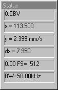
Active Trace Name
The name of the currently active trace is shown here on the status box. Use the TAB key to change the active trace. Use the Trace Properties box to change the name
ToolBar

The Tool Bar is a feature common to many Windows applications. It allows quick access to most of the more commonly used menu commands.
The tool bar is displayed across the top of the application window, below the menu bar. The tool bar provides quick mouse access to many tools used in CAM1,
Sometimes some of the Tool Bar buttons will be inactive ( dimmed ). Usually this is when the button is not applicable to the currently active window.
To hide or display the Tool Bar, choose Toolbar from the View menu (ALT, V, T).
Calculating Averages
Use this command to recalculate averages. This command is only available when data is selected.
Averages, minimum and maximum are entered into the most recently active Results file. If no result file is open then a new one is created automatically. Each new average calculation is appended to the Result file.
Data is taken from the active trace, from the leftmost selected point up to the rightmost point. Zero points are excluded from the average, but this can be changed using the Artifact Filter.
Dropout and noise artifacts can be excluded from the result by using the Artifact Filter.
Data can be selected from the result file and copied to any other Windows application. Perhaps the primary use will be to copy results into a spreadsheet application such as Excel.
Hide Trace
 Use this command to hide the currently active trace. The trace remains
active although it is hidden from view. Activating a hidden trace automatically
reveals it.
Use this command to hide the currently active trace. The trace remains
active although it is hidden from view. Activating a hidden trace automatically
reveals it.
Increase Brightness
 Use this command to increase the 'brightness' of the currently active Doppler spectrum.
This actually reduces the value associated with the brightest colour of the current palette.
This only effects the displaying of the spectrum in the current view, it does not alter the actual data.
Decrease Brightness
 Use this command to reduce the 'brightness' of the currently active
Doppler spectrum.
Use this command to reduce the 'brightness' of the currently active
Doppler spectrum.
This actually increases the value associated with the brightest colour of the current palette.
This only effects the displaying of the spectrum in the current view, it does not alter the actual data.
Smooth trace
 Use this command to apply a single pole RC filter to the selection
of the currently active trace.
Use this command to apply a single pole RC filter to the selection
of the currently active trace.
The Smoothing box allows the time constant to be selected.
The Artifact Filter controls the action to take for signal dropouts and noise spikes.
This command destroys the original data in the selection of the trace!
Trace properties
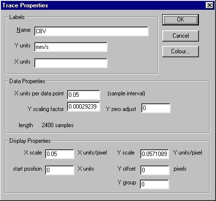
This dialog allows properties of the currently active trace to be altered.
This dialog can be invoked from the edit menu, or by clicking the right mouse button over a trace.
Y units
Y units of the active trace. This is a text string which can be edited by the user.
X units
The x units label. This is a text string which can be edited by the user.
Sample Rate
This shows the interval between samples in x units. Normally this should not be altered since it would have been set when the trace was recorded. (Or in the original trace from which this trace has been derived).
See also Data Rate.
Axes X scale
The scaling of the x units to screen pixels.
Trace Start Position
Alter this to shift the trace start position. Don't change the start positions of traces in the Monitor window.
Screen Y scale
The scaling of y units to screen pixels. Note that the Doppler spectrum y scale has to result in the trace being displayed as a power of 2 pixels high.
Screen Y offset
The offset used to shift the active trace in the y axis, in screen pixels. This value does not change with y scale changes. Easier to change by clicking the left mouse button on the y axis and dragging. (Set Y Group to -1 to offset just this trace.)
Y scaling factor
The scaling factor used to scale the stored data to the y axis scale.
Trace Selection Dialog
Select desired trace from list of all traces available. Some traces may be empty ( have been deleted using Edit command ) and some may not be appropriate for the operation. The command should fail safely if you make a bad choice.
View
Colour / mono Doppler spectrum
Use this command to switch all Doppler traces in all views between colour and monochrome display.
Remember to switch to mono before printing onto a mono printer.
Inverse Colours
This function reverses the colour coding of the Doppler spectrum. Useful for printing out onto non-colour printers, either to save ink or toner, or to improve the visual appearance.
Minimum to background
Use this set the colour of the lowest values to the same colour as the background. This is sometimes useful for printouts in order to either improve the appearance, or to conserve printer ink or toner.
Advanced Menu
This menu provides advanced functions, some of which are primarily for development purposes. To access this menu press [Ctrl]A.
WARNING: some of the undocumented functions do not have full error checking. Make sure important data is saved before using any of these commands.
Artifact Filter Dialog
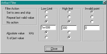
The Artifact Filter dialog controls the action (if any) to take when the signal is above or below the specified levels. Used by the Average and Smoothing commands.
The low limit is primarily used for excluding dropout signals from average calculations. The default value, and 'Set to zero and skip' should be suitable for many cases. The dropouts may be from loss of signal due to tissue movement or gaps in the erythrocytes passing through the capillary.
The high limit is primarily used for excluding noise spikes generally caused by laser reflections from the tissue surface. This is not as effective as the low level filter, since it is difficult to distinguish between the sharp rise from the cardiac pulse and noise. Using an absolute value on small sections at a time may be most appropriate.
To apply only the artifact filter to a trace, Smooth the trace using a zero time constant.
Artifact Limit
Enter a value here for the limit of acceptable values. Either absolute values or percent of the last valid value can be used.
Absolute Value
Set the limit to an absolute value. Units of the currently active trace in the current view are used. Any values above or below this will be considered as artifact. Action to be taken is set by the Filter Action.
Percent
The percentage of the last valid value is used as the artifact limit. All values above or below this level are treated as artifact.
Filter Action
No Action
Ignore this artifact limit and calculate all points.
Repeat last valid value
The last value within the artifact limits is substituted for points falling outside the artifact limits.
Set to zero & skip
If the output of the operation is a trace then the result for any points falling above or below the limits will be set to zero.
In the Smoothing operation the artifact value is ignored and does not influence the smoothed trace. (No compensation for the missing time is made).
For the Average calculations the point is simply ignored.