Step by Step Guide

Step 1. Displaying Video

Launch CapiScope by clicking on its icon. Start grabbing images by clicking on the Grab video button. You can adjust the Contrast and Brightness of the Input image using the Video Input control. Click on View on the menu and select Video Input control.

Change the video input gain by selecting from the list of available gains. Press the pan button. Click on the image and drag with the left mouse button. The image should move with the mouse.

Step 2. Dimension Lines

Click on the measurement button, and then click on the counting button. Then click on capillaries using the left mouse button. Each point has a number next to it. From the Windows menu, select Dimension List. This will open the dimension list window. Add some more points to the video window. Note how each new point is added to the dimension list.

Click on the dimension line button. Click the left mouse button on the image. Move to a new point and click to add a new node. Note how the cursor position is displayed in the second indicator pane in the status bar. The third indicator pane shows the x and y distance from the last node. To end the line double click the left mouse button or press escape. The start position and the total length is added to the dimension list.

Select Grey Level from the Window menu. This will open a Grey Level chart window. Go back to the Live Video window and add a dimension new line. Notice how the grey level profile along the line is displayed in the Grey Level window. Note too that it is updated twice per second. Press the button to freeze the image. Click on the first point on any dimension line. This now becomes the active line (all nodes on the line will be shown as crosses), and the grey level profile will be shown in the Grey Level chart. Click on a dimension line and drag it by holding down the left mouse button, the Grey Level profile will be continuously updated as the line is moved.

Step 3. Diameter measurement

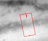
Draw a line perpendicular to a vessel. Right click on the first point of the line, and select Set line width from the pop-up menu. Set a width in pixels. In this image the width is 40 pixels.

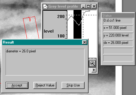
Click on the diameter measurement button. This will open the grey level window to show the grey level along the line, averaged over the width of the line. The detected vessel diameter is highlighted, and the dialog box shows the calculated vessel diameter.

To delete the active dimension line press the Delete key.

Step 4. Measurements

Click on the Region of Interest (ROI) button. Click and drag the mouse whilst holding down the left mouse button. This will create a region of interest. The size of the ROI will be displayed in the status bar as it is drawn. To see the size again, click on the ROI button. To move the ROI click on the ROI and drag while holding down the left mouse button. To calculate the number of capillaries and length of capillaries within the ROI press the button. This will open the Image Results window. Add more counts or lines to the image, or move or create a new ROI. Press the calculate button again. The new results will be added to the Image Results window. Click on the Show grid button to display the grid. Press it again to remove the grid. The grid size can be adjusted using the Settings | Grid menu option. Click the origin button. Now click the left mouse button on the image. The grid will now be aligned with the new origin, and the start positions in the dimension list will now be relative to the new origin. Double click the right mouse button on the image. This now will reset the position of the target crosshair.

Step 5. Notes

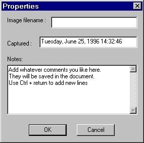
Select Notes… from the Edit menu. The Properties dialog will be shown:

Add whatever comments you like to the notes edit box. The image will be automatically given a filename when the document is saved for the first time. Only change this if you require a separate name for the image.

Step 6. Saving

Press the File Save button. If you have a Region of Interest (ROI) a prompt will ask if you want to save just the ROI or the whole image. Enter a new filename, eg test. CapiScope will create a CapiScope file test.cs1, and an image file test.kkg. Whenever test.cs1 is loaded, CapiScope will look for test.kkg and load that as the corresponding image. CapiScope will ask if you want to open the newly created file. Press No this time. Select File Open, and open the test.cs1 image. This should load the test.kkg image and all the dimensions previously saved.

Step 7. Video

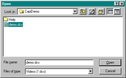
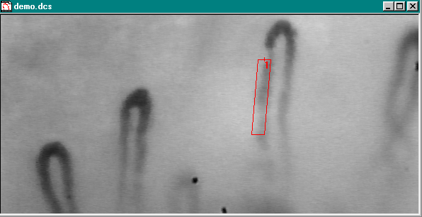
Open a video sequence file using file, Open… and choosing file types of Videos (.dcs)*.

The demo.dcs file in the capidemo directory on the CD is a good example.

See which direction the blood flow is travelling using the play () button.

Draw a line on a vessel as described above, following the direction of flow.

If you make any mistakes whilst drawing the line then just click on the first point of the line and press the Del key on the keyboard.

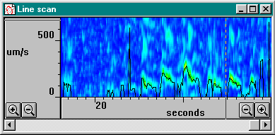
Click on Window, Linescan.to open the linescan window, which will be used to calculate the velocity.

Click on the title bar of the video window to reactivate it, then press the play () button again, this time the velocity will be calculated as the video sequence is played.

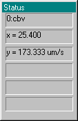
Click on the title bar of the linescan window to reactivate it, then press the TAB key, until the status box shows that the “cbv” trace (black trace) is activated. Spot measurements of capillary cell velocity can be read off from here.

Step 8. Velocity

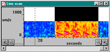
You can measure the average velocity by marking a section of the trace by dragging the mouse with the left mouse button held down.

Press the equals (=) key or button to calculate the average cbv over the marked period.

Note that periods where the correlation is poor, cbv is set to zero, and zero points, are, by default, excluded from the average result. The ratio of data points with good correlation to poor correlation is shown in the % used column.

The coloured trace in the linescan window is a correlellogram trace. High correlation is shown as red, and low correlation as blue, with a rainbow spectrum for values in between. Velocity is on the vertical axis.