Velocity Measurement¶

Theory¶

The dynamic capillaroscopy option enables capillary blood cell velocity to measured from live or recorded video using a spatial correlation technique.

Measurements can be made in real time, directly from the subject. However, it is usually more convenient to record onto good quality video tape or, for best quality, directly into the computer memory, or for longer sequences, directly to the hard disk. This also allows more than one vessel to be measured from the same image sequence. Note that the digitised video is not compressed, and will use about 10 Mbyte per second for a full frame.

Velocity is measured by using the mouse to draw a line along the vessel. The vessel can have any orientation, and does not even need to be straight, although straight vessels are more likely to give good results. The line thickness can be adjusted so that it covers the width of the capillary. This gives an average of the pattern over the whole width. i.e. the image of the vessel is projected onto a 1 pixel thick line. Note that the image itself has already effectively projected 3D into a 2D image (thicker vessels appear darker), and the averaging across the width of the vessel reduces the 2D information down to 1 dimension.

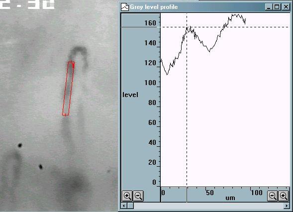
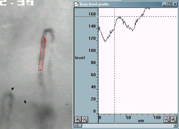
The grey level profile along the line is taken for each field every 1/50th of a second (1/60th second for NTSC based systems). Note that standard video formats have 25 (or 30) frames per second, but each frame is made from 2 interlaced fields. Even numbered lines make the even field, and odd numbered lines make the odd field. Usually, each field is captured separately and then sent whilst the next field is being captured.

The grey level pattern along each line is compared to the pattern from the next field (or several fields later for very low velocities).

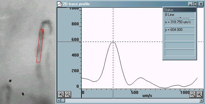
The comparison is performed by calculating the correlation coefficient for every possible shift of the previous grey level profile relative to the new profile. The shift which produces the highest correlation, and which can be seen as the peak in the correlation (the y scale is multiplied by 1000) in the following figure, indicates the distance that the pattern travelled between the two grey level profile measurements.

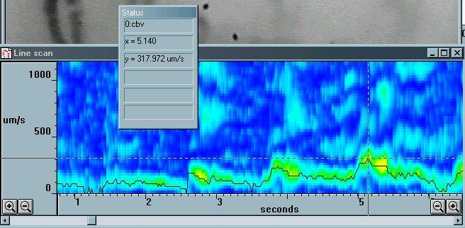
Since the time lapse between the two grey level profiles is known (ie 1/50th second) the velocity is easily calculated. CapiScope displays the correlation, along with the velocity trace (cbv) as a colour map, showing red for a high correlation through to blue for low correlation. If the correlation is below a preset limit then it is rejected, and a zero cbv value is set at that point.

Making Velocity Measurements¶

Measurement Line¶

The velocity calculation requires a measurement line. Most of the time, CapiScope can determine which line to use, but in the case of several dimension lines, or several video sequences open at the same time, you will need to specify which line to use.

Right click on the first node of the line. This should open a small menu. Click on “measurement line” to make this line the current measurement line.

Warning

All data in the linescan window will be lost without warning when switching to another line.

There are a few points to consider when creating measurement lines.

Maximum velocity is half the line length multiplied by number of fields per second (i.e. 50 or 60). This is reduced if the Set sample rate or number of Linescan sample periods between correlations are not both 1.
A straight line avoids the distortions which occurs at bends.
Horizontal lines have twice the resolution as vertical lines for interlaced video.
Using a line which is wider than the vessel, might help when there are movement artefacts, but the signal, and hence correlation will be poorer, since it will be averaged with useless background information.

If the vessel is large (> 30 um) then make the line cover only the central third of the vessel, otherwise the correlation will tend to pick out the slower rolling leukocytes along the vessel wall.
The line needs to be at least twice as long as typical pattern (erythrocyte gap or leukocyte). Note that the resolution of the cbv velocity measurement is half the length of the measurement line.

Movement¶

It is important to have no movement in the video sequence. If the subject moves, it is possible to reposition the line by dragging the first node of the measurement line using the mouse and left mouse button. This can be done whilst the sequence is running, or by stopping the video sequence, repositioning the measurement line, then resuming the sequence by clicking on the play button. See Calculate Movement Correction

Linescan input settings¶

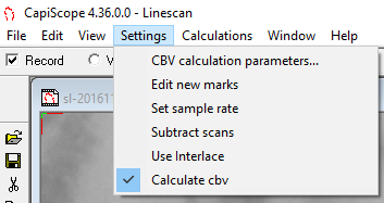
There are several settings which control and effect the capture of the video data for the velocity correlation measurements. These are found in the Settings menu whilst the Linescan window is active.

Calculate cbv¶

This menu item needs to be checked to enable cbv calculation in the linescan window. If it off, then only the grey level pattern along the line is recorded.

Subtract scans¶

This can be used for most measurements except very slow flows. When checked each grey level profile is subtracted from the grey level profile of the previous field. This removes any static pattern which might give an overwhelming zero velocity correlation. The newer high pass option in the CBV calculation parameters will give more options and also can be switched on/off without having to resample the video.

Set sample rate¶

The grey level profile along the line is, by default, sampled on every field of the video sequence. This setting allows a lower sampling rate for lower velocity measurements. It is recommended to leave this at the default value of 1 unless you are measuring for a long period (e.g. directly from the “live video” window with truly live video or from video tape) and so need to reduce the memory requirements of the linescan window.

Use Interlace¶

When ON, this option will sample the ODD lines, and then the EVEN lines so producing two linescans per video frame. This will effectively double the maximum velocity range when used with interlaced video.

CBV calculation parameters¶

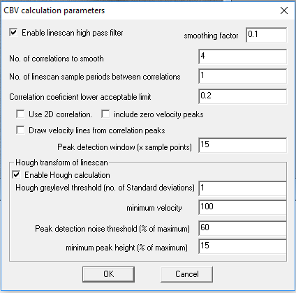
This dialog box enables fine tuning of the velocity measurement. Correlation and velocity will be recalculated when clicking on OK.

Number of correlations to smooth¶

This provides a smoothing function to the correlations. Without smoothing, the cbv trace would have many intermittent short spikes. Increasing the number of correlations smoothed, reduces the peak correlation coefficient. Therefore the correlation coefficient limit will need to be adjusted to a lower value.

Linescan sample periods between correlations¶

Increase this value for lower velocities, to improve resolution. Use an even number for interlaced video so that correlations are performed on the same ODD or EVEN field.

Correlation coefficient lower acceptable limit¶

Use this parameter to remove noise from low correlations. Values below this limit will give an invalid cbv value. Note that invalid values are not included in the average calculations (but this can be changed see artefact filter).

Use 2D correlation¶

When OFF, the grey level across the width of the linescan dimension line is averaged to give a single value for each pixel along the dimension line. These are the values used for the high pass filter and the correlation.

When ON, the grey level for each pixel across the width is used in the high pass filter and the correlation. If the vessel is not straight, and the linescan dimension line is wider than the vessel, then there will be a detrimental effect on the correlation .

Include zero velocity peaks¶

When OFF then detection of the correlation peak will ignore the peak at zero velocity.

When ON, then the zero peak will also be included in detection of the maximum peak.

Draw velocity lines from correlation peaks¶

Enable automatic drawing of velocity slope lines. Peaks in the correllogram are used to draw the lines.

Enabling this option automatically disables the Hough transform.

Peak detection window¶

Window width used for detecting maxima in the correlation trace. Value is width in x data points. Only one velocity line will be drawn for the window width.

Hough Transform linescan¶

This enables automatic detection of velocity slope patterns in the greylevel linescan.

This creates a Hough transform from the high pass filter of the linescan. Peaks in the Hough transform correspond to potential lines detected in the linescan. Velocity slopes are created from peaks found in the Hough transform.

Automatically turns off velocity slope drawing using the correllogram.

Hough greylevel threshold¶

This determines which pixels from the difference trace are candidates for line detection. The threshold value is the greylevel value above the average in multiples of standard deviation of the difference trace greylevel. A lower value will increase the number of pixels used and increase sensitivity but could also increase false detections.

Minimum Velocity¶

Velocity slopes below this value are ignored and not drawn.

Peak Detection Threshold¶

This is the minimum level considered as a peak in the Hough transform. Value is percentage of the maximum peak found in the Hough transform.

Minimum Peak Height¶

This sets the minimum peak height above surroundings before a peak is considered as a velocity line.

Average cbv vs correlation limit¶

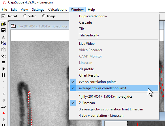Use the average cbv vs Correlation limit to open a plot of average cbv, maximum cbv, minimum cbv, and data points used vs correlation limit.

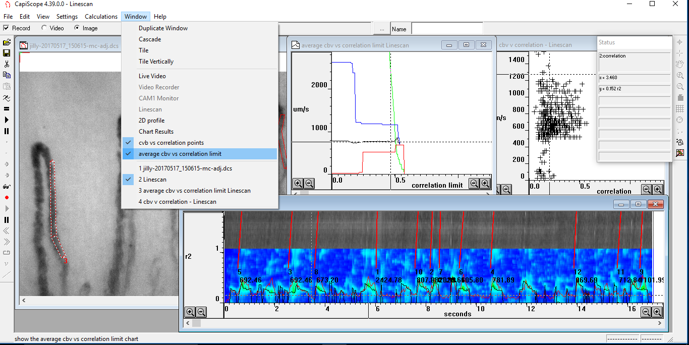
CapiScope calculates values for average cbv, maximum cbv, and minimum cbv for 250 different possible correlation limits from 0.0 upto 1.0. So for each point along the x-axis (correlation limit), only cbv values that are above that correlation limit are used for the average, maximum and minimum values.

Black trace = average cbv

Blue trace = maximum cbv

red trace = minimum cbv

green trace = number of data points above correlation limit

Use this chart to help determine the best correlation coefficient limit.

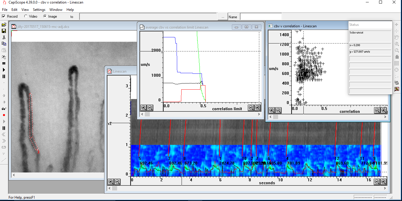
In the example below, we can see that there are some high maximum cbv values upto a correlation limit of about 0.2. Also there are low minimum cbv values upto a correlation limit of about 0.25.

The good news is that the average cbv is fairly flat. This means that the correlation limit used will not make a big change in the average cbv value.

We can also see that there are not many cbv values above a correlation limit of about 0.5. The green trace, showing the number of cbv points, falls rapidly at a correlation limit of about 0.5.

cbv vs correlation¶

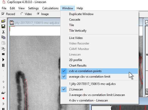
Use the cbv vs Correlation to open an x-y scatter plot of cbv vs correlation.

Each cbv value is plotted against the correlation value that produced it.